
Two-Way ANOVA: Formula, Examples, and How to Calculate It by Hand
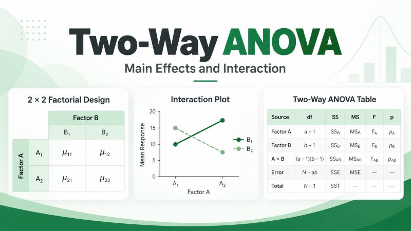
A two-way ANOVA is a statistical test used to determine whether two categorical independent variables have a significant effect on the mean of a quantitative dependent variable. For example, suppose a researcher wants to determine whether students’ examination scores differ according to both teaching method and study mode. A two-way ANOVA can test whether examination scores differ by teaching method, whether they differ by study mode, and whether the effect of teaching method depends on the study mode.
In this guide, we explain the two-way ANOVA, its main and interaction effects, hypotheses and formulas, how to calculate it by hand, and how to interpret and report the results.
What Is a Two-Way ANOVA?
A two-way ANOVA, also called a two-factor ANOVA, is used to examine the effect of two categorical independent variables on one quantitative dependent variable. The two categorical independent variables are referred to as factors, while the categories within each factor are called levels.
For example, suppose a researcher investigates whether examination scores are affected by:
- Teaching method: Lecture or Flipped Classroom
- Study mode: In-Person or Online
In this study:
- Teaching method is Factor A.
- Study mode is Factor B.
- Lecture and Flipped Classroom are the two levels of Factor A.
- In-Person and Online are the two levels of Factor B.
- Examination score is the quantitative dependent variable.
Because there are two factors, we can use a two-way ANOVA. The design in this example is called a 2 × 2 factorial design because Factor A has two levels and Factor B also has two levels. If Factor A had three levels and Factor B had two levels, it would instead be a 3 × 2 factorial design.
When Should You Use a Two-Way ANOVA?
Use a two-way ANOVA when you want to examine how two categorical independent variables are related to the mean of one quantitative dependent variable.
Generally, the following assumptions must be met:
- You have two categorical independent variables, also called factors.
- Each factor has two or more levels.
- You have one quantitative dependent variable.
- The observations are independent for an ordinary between-subjects two-way ANOVA.
- Your study includes observations for the combinations of the factor levels.
For example, suppose a crop researcher wants to determine whether crop yield differs according to fertilizer type and irrigation method.
The researcher may have:
- Factor A: Fertilizer type with three levels
- Factor B: Irrigation method with two levels
- Dependent variable: Crop yield
A two-way ANOVA would allow the researcher to test the effect of fertilizer, the effect of irrigation method, and whether the effectiveness of a fertilizer changes depending on the irrigation method.
How Does a Two-Way ANOVA Work?
A two-way ANOVA examines three effects:
- The main effect of Factor A
- The main effect of Factor B
- The interaction effect between Factor A and Factor B
Suppose Factor A is teaching method and Factor B is study mode.
The main effect of teaching method asks: Do mean examination scores differ between teaching methods when averaging across the study modes?
The main effect of study mode asks: Do mean examination scores differ between study modes when averaging across the teaching methods?
The interaction asks a different question: Does the effect of teaching method on examination scores depend on the study mode?
This interaction is one of the main reasons for using a two-way ANOVA instead of conducting separate one-way ANOVAs.
Main Effects
A main effect describes the overall effect of one factor after averaging across the levels of the other factor.
For example, suppose the mean scores are:
| Teaching Method | In-Person | Online | Overall Mean |
|---|---|---|---|
| Lecture | 72 | 70 | 71 |
| Flipped Classroom | 84 | 76 | 80 |
When we examine the main effect of teaching method, we compare the overall mean for Lecture (71) with the overall mean for Flipped Classroom (80).
However, when we examine the main effect of study mode, we compare:
- In-Person mean = (72 + 84) / 2 = 78
- Online mean = (70 + 76) / 2 = 73
These are called marginal means because each factor mean is calculated after averaging over the levels of the other factor.
Interaction Effect
An interaction occurs when the effect of one factor changes depending on the level of the other factor.
Using the previous means, for In-Person students: 84 − 72 = 12. This implies that the Flipped Classroom method produces a 12-point higher mean than the Lecture method.
For Online students: 76 − 70 = 6. The difference is now only 6 points.
Therefore, the size of the teaching-method effect changes depending on the study mode.
A two-way ANOVA determines whether a difference like this is large enough relative to the unexplained variation in the data to be considered statistically significant.
How Is Variation Divided in a Two-Way ANOVA?
Like a one-way ANOVA, a two-way ANOVA tests mean differences by examining variation. However, instead of dividing the variation into only between-group and within-group components, the two-way ANOVA separates the total variation into four parts:
- Variation explained by Factor A
- Variation explained by Factor B
- Variation explained by the interaction between Factor A and Factor B
- Unexplained or error variation within the groups
Therefore: SSTotal = SSA + SSB + SSA×B + SSError
Where:
- SSA is the sum of squares for Factor A.
- SSB is the sum of squares for Factor B.
- SSA×B is the sum of squares for the interaction.
- SSError is the within-cell or unexplained sum of squares.
- SSTotal is the total sum of squares.
Each effect is then compared with the error variation using an F statistic. Therefore, a two-way ANOVA produces three F tests rather than one.
Two-Way ANOVA Hypotheses
Because a two-way ANOVA tests three effects, there are three sets of hypotheses. Suppose Factor A has a levels, and Factor B has b levels, the hypotheses are:
1. Hypotheses for Factor A
- Null Hypothesis, H₀: The Factor A population means are equal.
- Alternative hypothesis, H₁: At least one Factor A population mean differs.
2. Hypotheses for Factor B
- Null hypothesis, H₀: The Factor B population means are equal.
- Alternative hypothesis, H₁: At least one Factor B population mean differs.
3. Hypotheses for the Interaction
- Null hypothesis, H₀: There is no interaction between Factor A and Factor B.
- Alternative Hypothesis, H₁: There is an interaction between Factor A and Factor B.
A significant interaction indicates that the effect of one factor depends on the level of the other factor.
Two-Way ANOVA Formulas
To calculate a balanced two-way ANOVA with replication by hand, you need to calculate the sum of squares, degrees of freedom, mean square, and F statistic for each source of variation.
Let:
- a = number of levels of Factor A
- b = number of levels of Factor B
- n = number of observations in each cell
- N = total number of observations = abn
- x̄ᵢ.. = mean for level i of Factor A
- x̄.ⱼ. = mean for level j of Factor B
- x̄ᵢⱼ. = mean for the cell formed by levels i and j
- x̄… = grand mean
- xᵢⱼₖ = an individual observation in cell ij
In a balanced design, each combination of Factor A and Factor B contains the same number of observations.
Before completing the ANOVA table, first calculate the grand mean: x̄… = Σx / N. You can then calculate the remaining components using the following two-way ANOVA formulas.
| Source | Sum of Squares | df | Mean Square | F Statistic |
|---|---|---|---|---|
| Factor A | SSA = bnΣ(x̄ᵢ.. − x̄…)² | dfA = a − 1 | MSA = SSA / dfA | FA = MSA / MSError |
| Factor B | SSB = anΣ(x̄.ⱼ. − x̄…)² | dfB = b − 1 | MSB = SSB / dfB | FB = MSB / MSError |
| A × B Interaction | SSA×B = nΣΣ(x̄ᵢⱼ. − x̄ᵢ.. − x̄.ⱼ. + x̄…)² | dfA×B = (a − 1)(b − 1) | MSA×B = SSA×B / dfA×B | FA×B = MSA×B / MSError |
| Error | SSError = ΣΣΣ(xᵢⱼₖ − x̄ᵢⱼ.)² | dfError = ab(n − 1) | MSError = SSError / dfError | — |
| Total | SSTotal = Σ(x − x̄…)² | abn − 1 | — | — |
The total variation can also be obtained by adding the four components of variation: SSTotal = SSA + SSB + SSA×B + SSError
How to Calculate a Two-Way ANOVA by Hand
To calculate a two-way ANOVA manually, follow these general steps:
- State the hypotheses for Factor A, Factor B, and the interaction.
- State the significance level, α.
- Calculate the three F statistics. To do this:
- Calculate the cell means, factor means, and grand mean.
- Calculate the sum of squares for Factor A.
- Calculate the sum of squares for Factor B.
- Calculate the interaction sum of squares.
- Calculate the error sum of squares.
- Calculate the total sum of squares.
- Find the degrees of freedom and mean squares.
- Calculate the F statistics.
- Find the p-values or F critical values.
- Make a decision for each effect.
- Write the conclusions in the context of the problem.
Example
A university researcher wants to determine whether examination scores differ according to teaching method and study mode. Twelve students are assigned to the following four conditions:
| Teaching Method | Study Mode | Examination Scores |
|---|---|---|
| Lecture | In-Person | 70, 72, 74 |
| Lecture | Online | 68, 70, 72 |
| Flipped Classroom | In-Person | 82, 84, 86 |
| Flipped Classroom | Online | 74, 76, 78 |
At the 0.05 significance level, determine whether there is a significant effect of teaching method, study mode, or an interaction between teaching method and study mode.
Assume the conditions for a two-way ANOVA are satisfied.
Solution
To perform a two-way ANOVA for the above data by hand, follow these steps:
Step 1: State the Hypotheses
The hypotheses are:
Teaching method:
- H₀: Mean examination scores are equal between teaching methods.
- H₁: Mean examination scores differ between teaching methods.
Study mode:
- H₀: Mean examination scores are equal between study modes.
- H₁: Mean examination scores differ between study modes.
Interaction:
- H₀: There is no interaction between teaching method and study mode.
- H₁: There is an interaction between teaching method and study mode.
Step 2: State the Significance Level
We want to test each effect at the 0.05 significance level. Therefore, α = 0.05.
Step 3: Calculate the Test Statistics
We need to calculate an F statistic for teaching method, study mode, and their interaction. To do that, follow these substeps.
i) Calculate the Cell Means
Calculate the mean examination score for each combination of teaching method and study mode.
Lecture × In-Person: x̄₁₁ = (70 + 72 + 74) / 3
= 216 / 3
= 72
Lecture × Online: x̄₁₂ = (68 + 70 + 72) / 3
= 210 / 3
= 70
Flipped Classroom × In-Person: x̄₂₁ = (82 + 84 + 86) / 3
= 252 / 3
= 84
Flipped Classroom × Online: x̄₂₂ = (74 + 76 + 78) / 3
= 228 / 3
= 76
Therefore, the cell means are:
| Teaching Method | In-Person | Online |
|---|---|---|
| Lecture | 72 | 70 |
| Flipped Classroom | 84 | 76 |
ii) Calculate the Factor Means
Calculate the marginal mean for each level of Factor A.
Lecture: x̄Lecture = (72 + 70) / 2
= 71
Flipped Classroom: x̄Flipped = (84 + 76) / 2
= 80
Thus:
- Lecture mean = 71
- Flipped Classroom mean = 80
Now calculate the means for Factor B.
In-Person: x̄In-Person = (72 + 84) / 2
= 78
Online: x̄Online = (70 + 76) / 2
= 73
Thus:
- In-Person mean = 78
- Online mean = 73
iii) Calculate the Grand Mean
The grand mean is the mean of all 12 examination scores.
The sum of all the scores is: 70 + 72 + 74 + 68 + 70 + 72 + 82 + 84 + 86 + 74 + 76 + 78 = 906
Therefore, the grand mean, x̄… = 906 / 12
= 75.5
iv) Calculate the Sum of Squares for Factor A
Teaching method is Factor A. The sum of squares formula is: SSA = bnΣ(x̄ᵢ.. − x̄…)²
In this example:
- b = 2 study modes
- n = 3 observations per cell
Therefore, SSA = 2(3)[(71 − 75.5)² + (80 − 75.5)²]
= 6[(−4.5)² + (4.5)²]
= 6(20.25 + 20.25)
SSA = 243
v) Calculate the Sum of Squares for Study Mode
Study mode is Factor B. The sum of squares formula is: SSB = anΣ(x̄.ⱼ. − x̄…)²
Since:
- a = 2 teaching methods
- n = 3 observations per cell
We can calculate SSB as follows:
SSB = 2(3)[(78 − 75.5)² + (73 − 75.5)²]
= 6[(2.5)² + (−2.5)²]
= 6(6.25 + 6.25)
SSB = 75
vi) Calculate the Interaction Sum of Squares
The interaction sum of squares formula is: SSA×B = nΣΣ(x̄ᵢⱼ. − x̄ᵢ.. − x̄.ⱼ. + x̄…)²
We first calculate the interaction component for each cell.
- Lecture × In-Person: 72 − 71 − 78 + 75.5 = −1.5
- Lecture × Online: 70 − 71 − 73 + 75.5 = 1.5
- Flipped Classroom × In-Person: 84 − 80 − 78 + 75.5 = 1.5
- Flipped Classroom × Online: 76 − 80 − 73 + 75.5 = −1.5
Therefore, SSA×B = 3[(-1.5)² + (1.5)² + (1.5)² + (-1.5)²]
= 3(2.25 + 2.25 + 2.25 + 2.25)
= 27
vii) Calculate the Error Sum of Squares
The error sum of squares measures the variation of individual observations around their respective cell means.
Lecture × In-Person: (70 − 72)² + (72 − 72)² + (74 − 72)²
= 4 + 0 + 4
= 8
Lecture × Online: (68 − 70)² + (70 − 70)² + (72 − 70)²
= 4 + 0 + 4
= 8
Flipped Classroom × In-Person: (82 − 84)² + (84 − 84)² + (86 − 84)²
= 4 + 0 + 4
= 8
Flipped Classroom × Online: (74 − 76)² + (76 − 76)² + (78 − 76)²
= 4 + 0 + 4
= 8
Therefore, SS Error = 8 + 8 + 8 + 8
= 32
viii) Calculate the Total Sum of Squares
For a balanced two-way ANOVA, SSTotal = SSA + SSB + SSA×B + SSError
Therefore, SSTotal = 243 + 75 + 27 + 32
= 377
ix) Calculate the Degrees of Freedom
There are:
- a = 2 teaching methods
- b = 2 study modes
- n = 3 observations per cell
- N = 12 total observations
Therefore, we can calculate the degrees of freedom as follows:
Teaching method: dfA = a − 1
= 2 − 1
= 1
Study mode: dfB = b − 1
= 2 − 1
= 1
Interaction: dfA×B = (a − 1)(b − 1)
= (2 − 1)(2 − 1)
= 1
Error: dfError = ab(n − 1)
= 2(2)(3 − 1)
= 8
Total: dfTotal = N − 1
= 12 − 1
= 11
x) Calculate the Mean Squares
Teaching method: MSA = SSA/dfA
= 243 / 1
= 243
Study mode: MSB = SSB / dfB
= 75 / 1
= 75
Interaction: MSA×B = SSA×B / dfA×B
= 27 / 1
= 27
Error: MSError = SSError / dfError
= 32 / 8
= 4
xi) Calculate the F Statistics
We can now compute the F-statistic as follows:
Teaching method: FA = MSA / MSError
= 243 / 4
= 60.75
Study mode:
FB = MSB / MSError
= 75 / 4
= 18.75
Interaction: FA×B = MSA×B / MSError
= 27 / 4
= 6.75
Therefore:
- F Teaching Method = 60.75
- F Study Mode = 18.75
- F Interaction = 6.75
Step 4: Find the P-Values and F Critical Values
Each test has numerator df = 1 and denominator df = 8. Using the p-value from F calculator, the p-values for the F-statistics are:
- Teaching Method: F(1, 8) = 60.75, p < .001
- Study Mode: F(1, 8) = 18.75, p = .003
- Teaching Method × Study Mode: F(1, 8) = 6.75, p = .032
We can also obtain the critical value using the F critical value calculator or an F distribution table.
At α = 0.05 with df₁ = 1 and df₂ = 8, F critical = 5.3177
We can now complete the two-way ANOVA table as shown below.
| Source | SS | df | MS | F | p |
|---|---|---|---|---|---|
| Teaching Method | 243 | 1 | 243 | 60.75 | < .001 |
| Study Mode | 75 | 1 | 75 | 18.75 | .003 |
| Teaching Method × Study Mode | 27 | 1 | 27 | 6.75 | .032 |
| Error | 32 | 8 | 4 | — | — |
| Total | 377 | 11 | — | — | — |
Step 5: Make the Decisions
Teaching method: Since p < .001 is less than α = 0.05, we reject the null hypothesis for teaching method. We reach the same decision using the critical-value approach because the test statistic (F = 60.75) is greater than the F-critical value (5.3177).
Study mode: Since p = .003 is less than α = 0.05, we reject the null hypothesis for study mode. Similarly, since the F-statistic (18.75) is greater than the F-critical (5.3177), we reject the null hypothesis.
Interaction: Since p = .032 is less than α = 0.05, we reject the null hypothesis of no interaction. Similarly, since the test statistic (F = 6.75) is greater than F-critical (5.3177), we reject the null hypothesis.
Therefore, all three effects are statistically significant.
Step 6: Write the Conclusion
At the 0.05 significance level:
- There is sufficient evidence that mean examination scores differ according to teaching method and study mode.
- There is also a statistically significant interaction between teaching method and study mode.
This means that the effect of teaching method on examination scores depends on whether students study in person or online.
Because the interaction is statistically significant, this interaction should receive particular attention when interpreting the results rather than relying only on the two overall main effects.
You can verify these results by selecting Two-Way ANOVA in the ANOVA Calculator.
How to Interpret a Two-Way ANOVA
A two-way ANOVA gives you three hypothesis tests, and each one answers a different question. However, you should generally examine the interaction first.
1. Interpret the Interaction Effect
Look at the p-value for Factor A × Factor B. If p < α, the interaction is statistically significant. This indicates that the effect of one factor changes depending on the level of the other factor.
When the interaction is statistically significant, be careful when interpreting the main effects by themselves because an overall average can hide important differences among the individual factor combinations.
For example, an overall teaching-method effect may suggest that one teaching method produces higher scores. However, a significant interaction might reveal that the advantage is very large for in-person students but small or absent for online students.
In such situations, follow-up simple effects or appropriate pairwise comparisons can help determine where the differences occur.
2. Interpret the Main Effect of Factor A
If the interaction does not prevent a meaningful interpretation of the main effect, examine the p-value for Factor A. If p < α, reject the null hypothesis for Factor A. This indicates that the population means differ across the levels of Factor A after averaging across Factor B.
3. Interpret the Main Effect of Factor B
Next, examine the p-value for Factor B. If p < α, reject the null hypothesis for Factor B. This indicates that the population means differ across the levels of Factor B after averaging across Factor A.
Interaction Plots
An interaction plot provides a useful visual representation of how the two factors work together. One factor is normally placed on the horizontal axis, while separate lines represent the levels of the second factor.
If the lines are approximately parallel, this usually suggests little evidence of interaction. However, if the lines are clearly nonparallel or cross, this may suggest that an interaction is present.
Note. The graph alone should not be used to determine statistical significance. Use the F statistic and p-value from the interaction test to make the formal decision.
What Should You Do After a Significant Interaction?
If the interaction is statistically significant, the next step is often to examine simple effects. A simple effect examines one factor separately at a particular level of the other factor.
For example, after finding a significant Teaching Method × Study Mode interaction, you might compare:
- Lecture vs Flipped Classroom among In-Person students
- Lecture vs Flipped Classroom among Online students
Alternatively, you could compare:
- In-Person vs Online within the Lecture group
- In-Person vs Online within the Flipped Classroom group
Which comparisons are most appropriate should depend on the research question. If a factor contains more than two levels, multiple pairwise comparisons may also require an adjustment for multiple testing.
Two-Way ANOVA With Replication vs Without Replication
You may come across the terms two-way ANOVA with replication and two-way ANOVA without replication, particularly when using Excel. A two-way ANOVA has replication when there are multiple independent observations for each combination of Factor A and Factor B.
Consider the table below
| Teaching Method | Study Mode | Scores |
|---|---|---|
| Lecture | Online | 68, 70, 72 |
| Lecture | In-Person | 70, 72, 74 |
From the table, we can see that there are three observations in each cell. This means that this is a two-way ANOVA with replication. Having replication allows the ordinary factorial ANOVA to estimate the within-cell error and test the interaction between the two factors separately.
On the other hand, a two-way ANOVA without replication has only one observation for each Factor A × Factor B combination.
For example:
| Online | In-Person | |
|---|---|---|
| Lecture | 70 | 72 |
| Flipped Classroom | 76 | 84 |
With only one observation per cell, there is no separate within-cell estimate of random error. As a result, the traditional two-factor ANOVA without replication cannot separately estimate an interaction effect in the same way as a replicated factorial design. It generally relies on an additive model in which interaction is not estimated separately.
For most studies in which you specifically want to investigate an interaction, having replication is therefore important.
Balanced and Unbalanced Two-Way ANOVA
A balanced two-way ANOVA has the same number of observations in every Factor A × Factor B cell. The manual formulas shown earlier assume a balanced design. For example, if there are three observations for cells A₁B₁, A₁B₂, A₂B₁, and A₂B₂, the design is balanced.
However, real datasets often have unequal cell sizes. This is called an unbalanced design. Two-way ANOVA can still be performed with unequal sample sizes, but the sums of squares are no longer as simple to partition manually. Depending on the statistical method, Type I, Type II, or Type III sums of squares may be used.
For this reason, statistical software is usually preferable for an unbalanced factorial design.
The ANOVA Calculator can perform a two-way ANOVA from raw data and provides the main effects, interaction effect, effect sizes, follow-up comparisons, and interaction plot.
One-Way ANOVA vs Two-Way ANOVA
The main difference between one-way and two-way ANOVA is the number of categorical independent variables included in the analysis. The table below provides a quick summary of the key differences.
| Feature | One-Way ANOVA | Two-Way ANOVA |
|---|---|---|
| Number of factors | 1 | 2 |
| Quantitative dependent variables | 1 | 1 |
| Tests main effects | Yes | Yes, for both factors |
| Tests interaction | No | Yes |
| Example | Teaching method → exam score | Teaching method + study mode → exam score |
For example, suppose you want to compare examination scores across Lecture, Hybrid, and Flipped Classroom teaching methods. Since there is only one categorical independent variable, you would use a one-way ANOVA. However, if you want to examine teaching method and study mode simultaneously, a two-way ANOVA is appropriate.
Want to learn more about a one-way ANOVA? See the complete guide on how to find a one-way ANOVA by hand.
Two-Way ANOVA Assumptions
Before performing an ordinary two-way ANOVA, consider the following assumptions.
1. Independent Observations
The observations should be independent. For a standard between-subjects two-way ANOVA, one participant’s measurement should not determine another participant’s measurement, and the same observation should not simply be repeated across multiple independent cells. If the same participants are measured repeatedly, a repeated-measures or mixed-design ANOVA may be more appropriate.
2. Quantitative Dependent Variable
The dependent variable should be quantitative. Examples include examination score, blood pressure, crop yield, waiting time, or income. However, the two independent variables should be categorical.
3. Approximate Normality
The dependent variable, or more specifically the model residuals within the factor combinations, should be approximately normally distributed. This assumption becomes particularly important when cell sample sizes are small.
You should also investigate strong outliers because they can substantially influence group means and the error variance.
4. Homogeneity of Variances
The population variances should be reasonably similar across the Factor A × Factor B groups. This is called the homogeneity of variance assumption. To assess this assumption, you should use Levene’s test.
5. Appropriate Study Design
The observations should correspond to the factorial structure being analyzed. For example, if you are testing teaching method and study mode, the data should clearly identify the teaching method and study mode associated with every examination score.
How to Report a Two-Way ANOVA in APA
When reporting a two-way ANOVA, report the results for:
- Factor A
- Factor B
- Factor A × Factor B interaction
For each effect, the usual format is: F(df₁, df₂) = F statistic, p = p-value. Using our worked example, we could report the interaction as: F(1, 8) = 6.75, p = .032
A suitable interpretation would be:
A two-way ANOVA showed a statistically significant interaction between teaching method and study mode on examination scores, F(1, 8) = 6.75, p = .032. The two main effects were also statistically significant: Teaching method, F(1, 8) = 60.75, p < .001 and Study mode, F(1, 8) = 18.75, p = .003.
However, because the interaction was statistically significant, the relationship between teaching method and examination scores should be interpreted in the context of study mode.
In a complete report, you may also report descriptive statistics, an effect size, and the results of any follow-up simple-effects or pairwise comparisons.
Want a tool that performs a two-way ANOVA and writes a complete APA report for you? Use the Two-Way ANOVA calculator.
Effect Size for a Two-Way ANOVA
Statistical significance tells you whether there is sufficient evidence of an effect, but it does not describe the size of that effect. A commonly reported effect size for factorial ANOVA is partial eta squared, written as partial η².
For an individual effect, partial η² = SS Effect / (SS Effect + SS Error)
For example, for the interaction in our worked example, partial η² = 27 / (27 + 32)
= 27 / 59
= 0.4576
This indicates the size of the interaction effect relative to the interaction plus error variation in the sample. You can use the same formula to calculate the effect size of Factor A and Factor B using their respective sums of squares.
Frequently Asked Questions
A two-way ANOVA is a statistical test used to examine how two categorical independent variables affect the mean of one quantitative dependent variable. It tests the main effect of each factor and the interaction between the two factors.
It is called a two-way ANOVA because the analysis contains two categorical independent variables or factors.
A two-way ANOVA normally tests three effects: the main effect of Factor A, the main effect of Factor B, and the Factor A × Factor B interaction.
No. A standard two-way ANOVA typically assumes independent observations. However, if the same participants are measured repeatedly across conditions, you may need a two-way repeated-measures ANOVA or a mixed ANOVA depending on the study design.
A main effect describes the overall relationship between one factor and the dependent variable after averaging across the other factor. On the other hand, an interaction determines whether that relationship changes across the levels of the other factor.
Yes. “Two-way” refers to the number of factors, not the number of groups or levels. For example, a study with three teaching methods and four age groups is still a two-way ANOVA because it contains two factors. It would be described as a 3 × 4 factorial design.
No. Modern statistical software can perform a two-way ANOVA with unequal cell sizes. However, unbalanced designs require more careful treatment of sums of squares and interpretation. The simple hand-calculation formulas shown in this guide are intended for a balanced design.
