
Want to perform a chi-square test of independence instead? Use the chi-square test calculator.
How to Use the Chi Square Goodness of Fit Calculator
This calculator helps you find the chi-square goodness-of-fit test either from raw data or summary data. To use the calculator:
- Select the correct Data Input Type. If you know how many observations fall within each category, select the Summary Data Option. However, if you have the individual categorical responses rather than summarized counts, select the Raw Data option
- Enter the significance level, α. You should enter your significance level as a decimal.
- Enter the variable name and the expected distribution. This calculator supports equal proportions, expected proportions, and expected counts
- Enter the data. For summary data, you’ll need to enter the category name, observed count, and expected proportions/counts if appropriate. However, for raw data, enter the categories and make sure to separate them using commas, line breaks, or semicolons. You can also paste raw values directly from Excel, Google Sheets, or text documents.
- Click Calculate
The calculator will instantly perform the chi-square goodness-of-fit test and return the χ² test statistic, its corresponding p-value, and critical value. It also provides a clear, step-by-step solution, showing you how to perform the test manually using the 6-step hypothesis test process.
Tips.
- Observed counts must be nonnegative whole numbers because they represent actual numbers of observations.
- Select Equal Proportions as the expected distribution when all categories are expected to occur equally often
- Select Expected Proportions when the expected distribution is unequal, and the question provides proportions or probabilities.
- Select Expected Counts when the expected number of observations in each category is already known.
Remember. The expected counts must add up to the observed sample size. Unlike observed counts, expected counts may contain decimals because they are calculated or theoretically predicted values.
What Is a Chi-Square Goodness-of-Fit Test?
A chi-square goodness-of-fit test is a statistical test used to test whether the observed distribution of one categorical variable differs significantly from a specified expected distribution.
It can help you answer questions such as:
- Are customers equally likely to choose four product designs?
- Do student majors follow the distribution reported by the university?
- Does the distribution of blood types in a sample match known population proportions?
- Are visits to a website equally distributed across the seven days of the week?
- Do genetic outcomes follow a specified inheritance ratio?
- Does the observed distribution of survey responses match the organization’s expected pattern?
The test compares the number of observations actually found in each category with the number that would be expected if the null hypothesis were true.
The hypotheses are:
- Null Hypothesis (H0). The data follows a specified distribution or set of proportions. In other words, any difference between real counts and expected counts happens only by random chance.
- Alternative Hypothesis (H1). The data does not follow the claimed distribution. In other words, we test to see whether at least one category’s true proportion is different from what was expected
When to Use a Chi-Square Goodness-of-Fit Test?
Use a chi-square goodness-of-fit test when:
- You have one categorical variable.
- The observations are recorded as category counts.
- Each observation belongs to only one category.
- You have a theoretical, historical, or otherwise specified expected distribution.
- You want to test the entire distribution rather than one category in isolation.
- The observations are independent.
- The expected counts are sufficiently large.
Conditions for a Chi-Square Goodness of Fit Test
To use the chi-square goodness of fit, the following conditions must be satisfied:
- The data must be counts or frequencies for one categorical variable
- The groups should be mutually exclusive such that each observation belongs to only one category
- The data must come from a random sample or a randomized experiment.
- Individual observations must be independent. Specifically, if sampling without replacement, the total sample size (n) must be less than 10% of the overall population (n ≤ 0.10N).
- All expected counts for every category must be at least 5.
Chi-Square Goodness-of-Fit Formula
The Pearson chi-square goodness-of-fit test formula is:
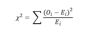
Where:
- χ2 is the chi-square test statistic.
- Oi is the observed count in category i.
- Ei is the expected count in category i.
How to Do a Chi-Square Goodness-of-Fit Test
Performing a chi-square goodness-of-fit test involves following the six steps of hypothesis testing. The following examples show how to perform the test using the manual method or our calculator.
Example 1. Finding the Test Manually
A large university bookstore claims that, historically, undergraduate students obtain their required textbooks according to the following probability distribution: 40% from the campus bookstore, 30% directly from the publisher’s website, 20% from an online marketplace (e.g., Amazon), and 10% through a textbook rental service.
A student government representative suspects that recent inflation and digital shifting have altered these purchasing habits. At the start of the Fall semester, she selects a simple random sample (SRS) of 200 undergraduate students and records their primary textbook sourcing method for the term. The observed results are summarized in the table below:
| Sourcing Method | Observed Count |
|---|---|
| Campus Bookstore | 104 |
| Publisher Website | 52 |
| Online Marketplace | 28 |
| Rental Service | 16 |
Perform an appropriate statistical test at the α = 0.05 significance level to determine if the current distribution of textbook-purchasing methods differs significantly from the historical baseline.
Solution
Since we have one categorical variable and we want to test whether the given sample data matches the historical baseline, the appropriate test is the chi-square goodness of fit test. To perform the test manually, follow these steps:
Step 1: State the Hypotheses
From the question, the historical expected proportions are: 0.40, 0.30, 0.20, and 0.10. Thus, we need to test the hypotheses:
- H₀: The data follow the specified population proportions (i.e., p1=0.40, p2=0.30, p3=0.20, p4=0.10).
- H₁: At least one population proportion differs from its historical value.
Step 2: State the Significance Level
We wish to test the hypothesis at a 0.05 significance level. Hence, α = 0.05
Step 3: Calculate the Chi-Square Statistic
By definition, the test statistic formula for the chi-square goodness of fit is: χ2 = Σ[(Oi − Ei)2/Ei]
From the question, we already know that the observed counts are:
- Campus bookstore: O1 = 104
- Publisher website: O2 = 52
- Online marketplace: O3 = 28
- Rental service: O4 = 16
Since we’re also given the expected proportions, we can find the expected count using the formula: Ei = npi, where n is the total sample size and pi is the expected population proportion.
Since n = 200, the expected counts are:
- Campus bookstore: E1 = 200 (0.40) = 80
- Publisher website: E2 = 200 (0.30) = 60
- Online marketplace: E3= 200(0.20) = 40
- Rental service: E4= 200(0.10) = 20
Substituting the values into the formula, we get:
χ2 = (104-80)2/80 + (52-60)2/60 + (28-40)2/40 + (16-20)2/20
= 7.2000 + 1.0667 + 3.6000 + 0.8000
= 12.6667
Therefore, the test statistic for the test is: χ2 = 12.6667
Step 4: Find the P-Value and Critical Value
To find the p-value or the critical value for the test, we first need to find the degrees of freedom. By definition, the degrees of freedom formula for a chi-square goodness-of-fit test is: df = k-1, where k is the number of categories.
Since there are 4 categories, df = 4-1
= 3
You can also use the degrees of freedom calculator to verify the above result.
To get the critical value for the test, we use the chi-square distribution table and find χ20.05, 3. This gives 7.8147. Want a quick solution? You can use the chi-square critical value calculator instead.
To find the p-value for the test, use the p-value calculator and follow these simple steps:
- Select the p-value from the chi-square statistic option
- Enter 12.6667 as the test statistic and df = 3
- Click calculate
The calculator will instantly return the p-value as 0.005416.
Step 5: Make the Decision
- Critical value approach. Since the test statistic (12.6667) is greater than the critical value (7.8147), we reject the null hypothesis (H0).
- P-value Approach. Since the p-value (0.005416) is less than the 0.05 significance level, we reject the null hypothesis (H0).
Step 6: Write the Conclusion
At the 5% significance level, there is sufficient evidence to conclude that the current distribution of textbook-purchasing methods differs from the historical distribution.
Example 2. Finding the Test using the Calculator (Summary Data)
Example 1 above is a good exam-style question you can solve using the Summary Data option of the chi-square goodness of fit test calculator. To perform the test using the calculator:
- Select the Summary Data option
- Enter the significance level as α = 0.05
- Enter the variable name as “Sourcing Method” and select expected proportions from the dropdown
- Key in the category names, observed counts, and expected proportions as shown in the table below
- Click calculate
| Category | Observed count | Expected proportion |
|---|---|---|
| Campus bookstore | 104 | 0.40 |
| Publisher website | 52 | 0.30 |
| Online marketplace | 28 | 0.20 |
| Rental service | 16 | 0.10 |
The calculator will instantly return the test statistic, p-value, and critical value, as follows:
- χ2 =12.6667
- P-value = 0.005416
- Critical value = 7.8147
As you can see, the results are similar to the manual solution. The calculator will also provide a clear, step-by-step solution explaining how to perform the test using the same data.
Example 3: Finding the Test Using the Calculator (Raw Data)
The Student Affairs Office at a large university wants to determine whether incoming first-year students are equally likely to choose among four primary study locations on or around campus: the Library, Residence Hall, Student Center, or Off Campus.
A simple random sample (SRS) of 40 first-year students was selected. The raw responses from the survey are provided below:
Library, Residence Hall, Library, Student Center, Library, Off Campus, Library, Residence Hall, Library, Student Center, Residence Hall, Library, Library, Residence Hall, Off Campus, Library, Student Center, Library, Residence Hall, Library, Student Center, Library, Residence Hall, Library, Off Campus, Residence Hall, Library, Student Center, Library, Residence Hall, Library, Off Campus, Student Center, Library, Residence Hall, Library, Student Center, Residence Hall, Library, Residence HallConduct an appropriate statistical test at the 5% significance level to determine if there is a significant difference in preference among the four study locations
Solution
To perform the test using the chi-square goodness of fit calculator, follow these steps:
- Select the Raw Data option
- Enter 0.05 as the significance level
- Enter the variable name as “Primary Study Location” and choose Equal Proportions from the dropdown (since we don’t have expected counts/proportion).
- Copy and paste the values into the raw data input field
- Click calculate
The calculator will automatically detect the four categories, the observed counts, and perform the chi-square goodness of fit test. It will instantly return the test statistic, p-value, and critical value as follows:
- χ² = 11
- P-Value = 0.011726
- Critical Value = 7.8147
The calculator will also provide a step-by-step solution explaining how to solve the problem manually.
Chi-Square Goodness of Fit vs Test of Independence
While the chi-square goodness of fit and test of independence use the same test statistic formula, they differ in various aspects. The table below provides a quick summary of the major differences between these two tests.
| Feature | Goodness-of-fit test | Test of independence |
|---|---|---|
| Number of variables | One categorical variable | Two categorical variables |
| Main question | Does the observed distribution match an expected distribution? | Are the variables associated? |
| Data structure | One set of category counts | Contingency table |
| Expected counts | Based on specified proportions or counts | Calculated from row and column totals |
| Degrees of freedom formula | df = k−1, where k is the number of categories | df = (r−1)(c−1), where r is the number of rows and c the number of columns in the contingency table. |
Frequently Asked Questions
It calculates Pearson’s chi-square goodness-of-fit test for one categorical variable. The results include the chi-square statistic, p-value, and critical value. The calculator also provides a clear, step-by-step solution showing you how to perform the test manually using your own data.
Select Expected Proportions when your expected values are probabilities expressed as decimals that total 1. However, if the predicted frequency for each category is already known and the counts total the observed sample size, Select Expected Counts.
Equal proportions means that every category is expected to have the same probability. With four categories, each expected proportion is 0.25. With five categories, each expected proportion is 0.20.
Yes. Raw-data mode of the calculator accepts individual categorical responses and counts the number of observations in each detected category automatically.
The degrees of freedom formula for a chi-square goodness of fit test is: df = k-1, where k is the number of categories.
