
How to Use the Skewness Calculator
This calculator helps you find the skewness of sample or population data. It also provides a clear interpretation of the result to help you determine whether your data is left-skewed, right-skewed, or approximately symmetric. To use the calculator:
- Choose whether your values represent sample data or population data.
- Enter your data values in the data input field. You can separate values using commas, spaces, tabs, or line breaks. The calculator also allows you to copy-paste values directly from Excel, Google Sheets, or text documents
- Click Calculate.
The calculator will instantly return the skewness value and tell you whether your data is positively skewed, negatively skewed, or approximately symmetric. It will also provide a distribution curve to help you visualize the distribution of your data.
What Is Skewness?
Skewness is a measure of the asymmetry of a dataset. It tells you whether the values are balanced on both sides of the distribution or whether the data has a longer tail on one side.
A dataset can be:
- approximately symmetric,
- positively skewed, also called right-skewed,
- or negatively skewed, also called left-skewed.
Skewness is useful because it helps you understand the shape of your data, not just the center or spread.
Population Skewness Formula
The population skewness formula is:
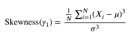
Where:
- γ1 is the population skewness.
- xi is each data value.
- μ is the population mean.
- σ is the population standard deviation.
- N is the total number of values in the population.
Sample Skewness Formula
For sample data, the skewness formula is:
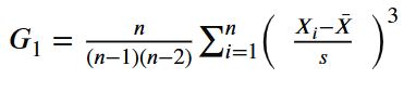
Where:
- G1 is the adjusted sample skewness.
- xi is each data value.
- x̄ is the sample mean.
- s is the sample standard deviation.
- n is the sample size.
Use the sample option when your dataset is only a sample from a larger population. This is the best choice for most classwork and research datasets.
Types of Skewness
There are three main types of skewness: positive skewness, negative skewness, and approximately symmetric distribution.
1. Positive Skewness
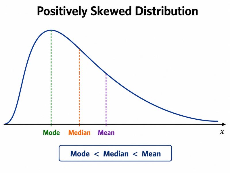
Positive skewness means the distribution has a longer tail on the right side. This is why positive skewness is often described as skewed to the right or right-skewed distribution.
In a positively skewed dataset, a few large values pull the mean to the right. As a result, the mean is often greater than the median. In other words, for a positively skewed distribution, the following relationship applies: Mode < Median < Mean
This pattern does not have to be perfect in every dataset, but it is a useful way to understand right-skewed data. The figure below shows a positively skewed distribution.
2. Negative Skewness
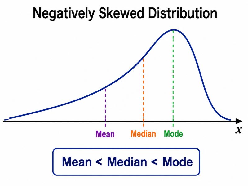
Negative skewness means the distribution has a longer tail on the left side. This explains why the negative skewness is also referred to as the skewed to the left or left skewness.
In a negatively skewed dataset, a few small values pull the mean to the left. As a result, the mean is often less than the median.
A common relationship for a negatively skewed distribution is: Mean < Median < Mode. The figure below shows a negatively skewed distribution demonstrating this relationship.
3. Approximately Symmetric Distribution
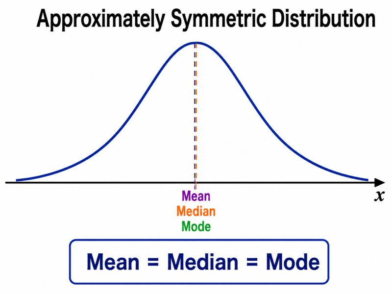
A distribution is approximately symmetric when the left and right sides are roughly balanced. In a real-world dataset, it is very unlikely to get a perfectly symmetric distribution. This is why we say an approximately symmetric distribution. In this case, the mean, median, and mode are usually close to one another.
A common relationship for an approximately symmetric distribution is: Mean ≈ Median ≈ Mode. It is worth noting that a symmetric distribution does not automatically prove that the data is perfectly normal. However, it suggests that the distribution is fairly balanced.
The figure below is a distribution curve showing the relationship between the mean, median, and mode in an approximately symmetric distribution.
How to Interpret Skewness Values
Have you just computed the skewness and not sure how to interpret it? The table below provides a quick summary of skewness values and their interpretations.
| Skewness value | Interpretation |
|---|---|
| Between -0.5 and 0.5 | The distribution is approximately symmetrical. The data is often treated as roughly normal, although normality should not be judged by skewness alone. |
| Between -1.0 and -0.5 or between 0.5 and 1.0 | The distribution is moderately skewed. |
| Between -2.0 and -1.0 or between 1.0 and 2.0 | The distribution is highly skewed. |
| Less than -2.0 or greater than 2.0 | The distribution shows substantial non-normality and may have severe outliers or a very long tail. |
Example
Suppose you have the following sample dataset: 5, 7, 8, 9, 10, 11, 12, 18. Find the skewness using the calculator and interpret the results.
Solution
To find the skewness of the dataset using the skewness calculator:
- Select the sample data option
- Copy and paste the values into the data input field
- Click Calculate
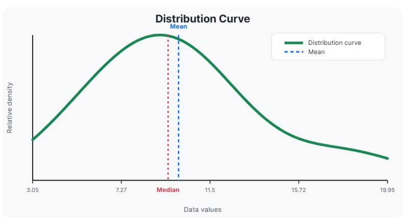
The calculator will instantly return: Skewness = 1.1315. Although the calculator provides the correct interpretation, we can use the above interpretation to arrive at similar interpretation.
Using the interpretation table, we can see that the skewness value of 1.1315 is between 1.0 and 2.0, which indicates that the distribution is highly skewed. Since the value is positive, we can say that the distribution is highly and positively skewed, or highly skewed to the right.
The distribution curve produced by the calculator also supports the interpretation by showing that the data is highly skewed to the right, as shown below.
Skewness and Normality
Skewness is often used to understand whether a dataset is close to symmetric. A skewness value near 0 suggests that the distribution is fairly balanced. However, skewness alone does not prove that data is normally distributed because some datasets can have low skewness and still not be normally distributed due to other features like unusual peaks, clusters, gaps, or heavy tails.
Therefore, you should never use skewness as the only test of normality. Instead, use it as a descriptive measure of shape and then follow up with other normality tests like the Shapiro-Wilk test or the Kolmogorov-Smirnov test.
Skewness vs Kurtosis
Although skewness and kurtosis are major descriptive statistics used in describing the visual shape of the data, they evaluate different data properties. In particular, skewness is a measure of asymmetry which tells us whether the distribution leans left or right, whereas kurtosis is a measure of tail heaviness, which tells us whether the distribution has unusually heavy or light tails.
Frequently Asked Questions
This calculator finds the skewness of sample or population data. It also explains whether the data is left-skewed, right-skewed, or approximately symmetric.
A positive skewness value means the data is right-skewed. In other words, the distribution has a longer tail on the right side.
A negative skewness value means the data is left-skewed. This means the distribution has a longer tail on the left side.
Skewness close to zero means the distribution is approximately symmetric. However, this does not always prove that the data is perfectly normal.
Yes. A skewness value greater than 1 usually suggests a highly positive skew. If it is greater than 2, the distribution may show substantial non-normality.
Yes. A skewness value less than -1 usually suggests a highly negative skew. If it is less than -2, the distribution may have substantial non-normality or a very long left tail.
