
Independent Samples T-Test: Formulas, Assumptions & Examples
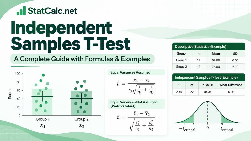
An independent samples t-test is a statistical hypothesis test used to determine whether the means of two independent populations differ significantly. For example, suppose a researcher wants to determine whether students taught using two different teaching methods have different mean examination scores. Since the students in one group are different from those in the other group, the researcher can use an independent samples t-test to compare the two population means.
There are two common versions of this test: the pooled independent samples t-test and Welch’s t-test. The pooled independent samples t-test assumes that the two populations have equal variances, while Welch’s t-test does not make this assumption.
In this guide, we explain when to use an independent samples t-test, its hypotheses and assumptions, the formulas for both versions of the test, and how to calculate each one by hand using complete examples.
Already knows the test and needs an online tool that performs the test and displays SPSS-style tables and APA report? Use the Independent Samples T-Test Calculator.
What Is an Independent Samples T-Test?
An independent samples t-test is a statistical test that compares the means of two separate and unrelated groups. It helps you determine whether there is a significant mean difference between two independent/unrelated groups.
Suppose μ₁ is the population mean for Group 1 and μ₂ is the population mean for Group 2. We take a sample from each population and calculate the corresponding sample means, x̄₁ and x̄₂. In most cases, the two sample means will not be exactly equal. This is expected because samples naturally vary.
Therefore, the important question is not simply whether x̄₁ and x̄₂ are different. Instead, we want to determine whether the observed difference is large enough relative to the expected sampling variability to provide evidence that the two population means differ.
The test does this by calculating a t statistic and then finding the probability of obtaining a result at least that extreme if the null hypothesis is true.
You may also come across the independent samples t-test under different names, including:
- independent t-test;
- independent sample t-test;
- unpaired t-test; and
- two-sample t-test.
These terms usually refer to the same general problem of comparing two independent population means. However, the formula changes depending on whether equal population variances are assumed.
When to Use an Independent Samples T-Test
Use an independent samples t-test when you want to compare the means of two independent groups.
For the test to be appropriate, the following conditions should be met:
- The dependent variable should be quantitative.
- The grouping variable should contain two separate groups.
- Each observation should belong to only one group.
- The observations in one group should be independent of those in the other group.
For example, suppose a researcher wants to compare examination scores between students taught using Method A and those taught using Method B. Examination score is the quantitative dependent variable, while teaching method is the grouping variable with two categories: Method A and Method B. Since different students make up the two groups, the observations are independent.
Other examples where you may use an independent samples t-test include the following:
- Comparing mean blood pressure between a treatment group and a control group.
- Comparing average salaries between employees in two departments.
- Comparing mean recovery times between patients receiving two different treatments.
- Comparing mean reaction times between participants assigned to two experimental conditions.
The key point is that you are comparing one quantitative outcome between two separate groups.
If you have only one sample and want to compare its mean with a specified or hypothesized value, use a one-sample t-test instead. You can perform the test directly using our One-Sample T-Test Calculator.
However, if the same participants are measured twice, such as before and after an intervention, the observations are related rather than independent. In that case, use a paired samples t-test or our Paired T-Test Calculator. If you need to compare the means of three or more independent groups, use a one-way ANOVA instead of performing several separate independent samples t-tests.
Hypotheses
For an independent samples t-test, the hypotheses for a two-tailed test are:
- Null hypothesis, H₀: The population mean for Group 1 is equal to the population mean for Group 2. In symbols, H₀: μ₁ = μ₂
- Alternative Hypothesis, H₁: The population mean for Group 1 is different from the population mean for Group 2. In symbols, H₁: μ₁ ≠ μ₂
You can also write the null hypothesis in terms of the difference between the two population means as follows: H₀: μ₁ − μ₂ = 0. This means that, under the null hypothesis, the population mean difference is assumed to be zero.
The alternative hypothesis may be two-tailed, right-tailed, or left-tailed depending on the research question. The table below shows the possible hypotheses.
| Type of Test | Research Question | Null Hypothesis | Alternative Hypothesis |
|---|---|---|---|
| Two-tailed | Are the population means different? | H₀: μ₁ = μ₂ | H₁: μ₁ ≠ μ₂ |
| Right-tailed | Is the Group 1 mean greater than the Group 2 mean? | H₀: μ₁ = μ₂ | H₁: μ₁ > μ₂ |
| Left-tailed | Is the Group 1 mean less than the Group 2 mean? | H₀: μ₁ = μ₂ | H₁: μ₁ < μ₂ |
Therefore, the alternative hypothesis you choose should match the research question. For example, suppose you want to determine whether students taught using Method A and Method B have different mean examination scores. Since the difference could occur in either direction, you would use a two-tailed test. In this case, the alternative hypothesis is: H₁: μ₁ ≠ μ₂
However, suppose the research question asks whether Method A produces a higher mean examination score than Method B. If Method A is Group 1, you would use a right-tailed test and the correct alternative hypothesis is: H₁: μ₁ > μ₂
Tip. The direction of the hypothesis should be decided before examining the test results.
Independent Samples T-Test Assumptions
Before performing an independent samples t-test, make sure your data and study design reasonably satisfy the assumptions below.
1. The Dependent Variable Should Be Quantitative
The dependent variable should be numerical and measured on a scale where calculating a mean is meaningful. Examples include examination scores, height, weight, income, blood pressure, reaction time, and temperature.
For example, if you want to compare examination performance between students taught using two teaching methods, examination score would be the quantitative dependent variable. A categorical outcome such as pass or fail would not be appropriate because calculating a mean for such categories would not be meaningful.
2. There Should Be Two Independent Groups
The grouping variable should contain two separate groups. For example, you may compare a treatment group with a control group, students taught using Method A with those taught using Method B, or participants assigned to two different experimental conditions.
Each participant should belong to only one of the two groups. If you want to compare the means of three or more independent groups, use ANOVA instead of performing several separate independent samples t-tests.
3. The Observations Should Be Independent
The observations in one group should not be related to observations in the other group. For example, if a student belongs to the Method A group, the same student should not also appear in the Method B group.
You normally determine whether this assumption is reasonable from the study design rather than from a statistical test. If the same participants are measured twice, such as before and after an intervention, the observations are related and a paired samples t-test would be more appropriate.
4. The Samples Should Be Randomly Selected or Reasonably Representative
Ideally, the samples should be randomly selected from the populations you want to study. Random sampling helps reduce selection bias and makes it easier to generalize the findings from the samples to the wider populations.
In practice, researchers do not always obtain perfectly random samples. However, the samples should still be reasonably representative of the populations of interest. A statistically significant t-test cannot correct serious problems caused by a biased sampling method.
5. The Data Should Be Approximately Normally Distributed for Small Samples
The dependent variable should be approximately normally distributed within each group, especially when the sample sizes are small. As the sample sizes increase, the independent samples t-test becomes more robust to moderate departures from normality.
This means that a small amount of skewness does not automatically make the test inappropriate, particularly with larger samples. However, strong skewness can still affect the sample means and standard deviations. As such, it is useful to examine the distributions using histograms, Q-Q plots, or other graphical methods.
6. The Data Should Not Contain Extreme Outliers
Extreme outliers can strongly affect the sample mean, standard deviation, and t statistic. For this reason, you should check each group for unusually large or small observations before performing the test.
A boxplot is a simple way to identify potential outliers. However, do not remove an observation simply because it appears unusual. First determine whether it is a genuine value or the result of a data-entry, recording, or measurement error. If the value is genuine, consider how much influence it has on the analysis before deciding how to proceed.
7. Equal Population Variances Are Required Only for the Pooled T-Test
The traditional pooled independent samples t-test assumes that the two populations have equal variances. In other words, the spread of values in one population should be reasonably similar to the spread in the other population.
If this assumption is reasonable, you can use the equal variances assumed version of the test. However, if the population variances cannot reasonably be assumed to be equal, use Welch’s t-test instead. Welch’s test does not require equal variances and adjusts the standard error and degrees of freedom accordingly.
Therefore, unequal variances do not mean that you cannot compare the two population means. They simply determine which version of the independent samples t-test is more appropriate.
Equal Variances Assumed vs Equal Variances Not Assumed
If you run an independent samples t-test in SPSS, the Independent Samples Test table normally reports two results:
- Equal variances assumed
- Equal variances not assumed
The Equal variances assumed row reports the pooled independent samples t-test, while the Equal variances not assumed row reports Welch’s t-test.
Our Independent Samples T-Test Calculator produces a similar SPSS-style output. When you enter raw data or upload a dataset, the calculator performs Levene’s test, reports both t-test results, and highlights the row you should interpret based on the Levene’s test result.
A common approach when interpreting SPSS output is to use Levene’s test as follows:
| Levene’s Test | Row Commonly Used |
|---|---|
| p ≥ .05 | Equal variances assumed |
| p < .05 | Equal variances not assumed |
For example, suppose Levene’s test gives p = .420. Since .420 > .05, there is not enough evidence to conclude that the population variances differ. Therefore, you would normally interpret the Equal variances assumed row.
However, suppose Levene’s test gives p = .012. Since .012 < .05, the equal variance assumption is not supported. In this case, you would use the Equal variances not assumed row, which reports Welch’s t-test.
Keep in mind that Levene’s test only helps you assess the equality of variances. It does not test whether the two population means are equal. After identifying the appropriate row, you still need to interpret the t statistic, degrees of freedom, and p-value to determine whether the population means differ.
Independent T-Test Formula (Equal Variance Assumed)
When equal population variances can reasonably be assumed, we use the pooled version of the independent samples t-test. The test statistic formula is:
Where:
- t is the independent samples t statistic.
- x̄₁ is the sample mean for Group 1.
- x̄₂ is the sample mean for Group 2.
- n₁ is the sample size for Group 1.
- n₂ is the sample size for Group 2.
- sₚ is the pooled sample standard deviation.
Since this version of the test assumes equal population variances, we first combine the two sample variances to estimate the common population variance. This gives the pooled variance. The pooled variance formula is:
Notice that we do not simply average the two sample variances. Instead, each variance is weighted by its degrees of freedom. If you only need to calculate this value, use our Pooled Variance Calculator.
Once the pooled variance is known, take its square root to get the pooled standard deviation. That is, sp = √sp2. You can also calculate this value directly from raw data or summary statistics using the Pooled Standard Deviation Calculator.
After calculating the test statistic, you also need the degrees of freedom to find the corresponding p-value or critical t value. When equal population variances are assumed, the degrees of freedom formula is: df = n₁ + n₂ − 2. If you do not want to calculate it manually, you can use our Degrees of Freedom Calculator for an instant result.
How to Calculate an Independent Samples T-Test by Hand (Equal Variances Assumed)
Example 1. A researcher wants to determine whether two teaching methods produce different mean examination scores. A random sample of 12 students taught using Method A has a mean score of 82 and a sample standard deviation of 7. Another independent sample of 12 students taught using Method B has a mean score of 76 and a sample standard deviation of 6.
Assume equal population variances. At the 0.05 significance level, is there enough evidence to conclude that the population mean scores differ?
Solution
Step 1: State the Hypotheses
The researcher wants to determine whether the two population means differ in either direction. Therefore, this is a two-tailed test.
We test:
- H₀: μ₁ = μ₂
- H₁: μ₁ ≠ μ₂
Step 2: State the Significance Level
From the question, the significance level, α = 0.05
Step 3: Calculate the T Statistic
Since equal population variances are assumed, the test statistic formula is:
From the question, we know that:
- x̄₁ = 82
- x̄₂ = 76
- s₁ = 7
- s₂ = 6
- n₁ = 12
- n₂ = 12
We first need to calculate the pooled variance and then the pooled standard deviation.
By definition, the pooled variance formula is:
Substituting the values gives:
= (539 + 396) / 22
= 42.5
Therefore, the pooled variance is sₚ² = 42.5.
To find the pooled standard deviation, we take the square root of the pooled variance.
Therefore, sₚ = √42.5
= 6.5192
We now have all the values needed to calculate the t statistic. Using the pooled independent samples t-test formula and substituting the values, we get:
= 6 / [6.5192 × √0.166667]
= 6 / 2.6615
Hence, t = 2.2544
Step 4: Find the P-Value and Critical Value
Before finding the p-value or critical t value, we need to calculate the degrees of freedom. The degrees of freedom formula is: df = n₁ + n₂ − 2.
Substituting the values, df = 12 + 12 − 2
= 22
Now, using the P-Value from T Calculator, the two-tailed p-value for t = 2.2544 and df = 22 is: p = 0.034463
We can also find the two-tailed critical value using the T Critical Value Calculator. For α = 0.05 and df = 22, t critical = ±2.0739
Step 5: Make the Decision
- P-value approach: Since the p-value (0.034463) is less than the 0.05 significance level, we reject the null hypothesis.
- Critical value approach: Since the absolute value of the calculated t-statistic (2.2544) is greater than the absolute t-critical value (2.0739), we reject the null hypothesis.
Step 6: Write the Conclusion
At the 0.05 significance level, there is sufficient evidence to conclude that the population mean examination scores differ between students taught using Method A and Method B. Method A had the higher sample mean, with an average score of 82 compared with 76 for Method B.
You can verify the calculation using our Two-Sample T-Test Calculator.
Independent T-Test Formula (Equal Variances Not Assumed)
When equal population variances cannot reasonably be assumed, we use Welch’s t-test. Welch’s t-test still compares the means of two independent populations, and the hypotheses remain the same. However, unlike the pooled t-test, it does not combine the two sample variances into a single estimate.
The Welch t-test statistic formula is:
Where:
- t is the independent samples t statistic.
- x̄₁ is the sample mean for Group 1.
- x̄₂ is the sample mean for Group 2.
- s₁ is the sample standard deviation for Group 1.
- s₂ is the sample standard deviation for Group 2.
- n₁ is the sample size for Group 1.
- n₂ is the sample size for Group 2.
Notice that there is no pooled variance or pooled standard deviation in the formula. Instead, the variance from each group is included separately. This makes Welch’s t-test useful when the two groups have different variances, different sample sizes, or both.
After calculating the test statistic, you also need the degrees of freedom to find the corresponding p-value or critical t value. Unlike the pooled t-test, Welch’s t-test uses the following degrees of freedom formula:
The resulting degrees of freedom do not have to be a whole number. For example, you may obtain df = 11.25. This is normal when performing Welch’s t-test.
How to Calculate an Independent Samples T-Test by Hand (Equal Variances Not Assumed)
Example 2. A researcher wants to determine whether two independent groups have different mean examination scores. Group 1 contains 10 students with a mean score of 82 and a sample standard deviation of 12. Group 2 contains 14 students with a mean score of 72 and a sample standard deviation of 5.
Assume equal population variances cannot be assumed. At the 0.05 significance level, is there enough evidence to conclude that the population mean scores differ?
Solution
Step 1: State the Hypotheses
The researcher wants to determine whether the two population means differ in either direction. Therefore, this is a two-tailed test.
We test:
- H₀: μ₁ = μ₂
- H₁: μ₁ ≠ μ₂
Step 2: State the Significance Level
From the question, the significance level, α = 0.05
Step 3: Calculate the T Statistic
Since equal population variances cannot be assumed, we use Welch’s t-test. The test statistic formula is:
From the question, we know that:
- x̄₁ = 82
- x̄₂ = 72
- s₁ = 12
- s₂ = 5
- n₁ = 10
- n₂ = 14
Substituting the values gives:
= 10 / √(144/10 + 25/14)
= 10 / √16.1857
t = 2.4856
Step 4: Find the Degrees of Freedom, P-Value, and Critical Value
Before finding the p-value or critical t value, we need to calculate the degrees of freedom. For Welch’s t-test, the degrees of freedom formula is:
Substituting the values gives:
= (14.4 + 1.7857)² / [(14.4² / 9) + (1.7857² / 13)]
= 261.9773 / 23.2853
Hence, df = 11.2508
Now, using the P-Value from T Calculator, the two-tailed p-value for t = 2.4856 and df = 11.2508 is approximately p = 0.029838. We can also find the two-tailed critical value using the T Critical Value Calculator. For α = 0.05 and df = 11.2508, the critical t value is approximately ±2.1950.
Step 5: Make the Decision
- P-value approach: Since the p-value (0.029838) is less than the 0.05 significance level, we reject the null hypothesis.
- Critical value approach: Since the absolute value of the calculated t statistic (2.4856) is greater than the absolute critical t value (2.1950), we reject the null hypothesis.
Step 6: Write the Conclusion
At the 0.05 significance level, there is sufficient evidence to conclude that the population mean examination scores differ between the two groups. Group 1 had the higher sample mean, with an average score of 82 compared with 72 for Group 2.
You can verify the calculation using our Welch’s T-Test Calculator.
Independent T-Test Confidence Intervals
An independent samples t-test can also be used to estimate the difference between two population means. This is done using a confidence interval for the mean difference.
The general form of the confidence interval is: CI = (x̄₁ − x̄₂) ± t critical × standard error
The standard error is the denominator used in the corresponding t-test formula. Therefore, its calculation depends on whether equal population variances are assumed or not.
A confidence interval also helps us interpret the hypothesis test. If the interval does not include zero, the two population means are significantly different at the corresponding significance level. However, if zero falls within the interval, there is not enough evidence to conclude that the population means differ.
1. Equal Variances Assumed
When equal population variances are assumed, the standard error, SE= sₚ × √(1/n₁ + 1/n₂).
Therefore, the confidence interval formula becomes: CI = (x̄₁ − x̄₂) ± t critical × [sₚ × √(1/n₁ + 1/n₂)]
In Example 1, we found that:
- x̄₁ = 82
- x̄₂ = 76
- sₚ = 6.5192
- n₁ = 12
- n₂ = 12
- df = 22
- t critical = 2.0739
Substituting these values gives:
CI = (82 − 76) ± 2.0739[6.5192 × √(1/12 + 1/12)]
= 6 ± 2.0739(2.6615)
= 6 ± 5.5195
Therefore, 95% CI = [0.4805, 11.5195]
This means we are 95% confident that the population mean score for Method A is between approximately 0.48 and 11.52 points higher than the population mean score for Method B.
Notice that zero is not included in the confidence interval. This agrees with the hypothesis test, where we rejected the null hypothesis.
2. Equal Variances Not Assumed
When equal population variances cannot be assumed, the standard error, SE = √(s₁²/n₁ + s₂²/n₂).
Therefore, the confidence interval formula becomes: CI = (x̄₁ − x̄₂) ± t critical × √(s₁²/n₁ + s₂²/n₂)
In Example 2, we found that:
- x̄₁ = 82
- x̄₂ = 72
- s₁ = 12
- s₂ = 5
- n₁ = 10
- n₂ = 14
- df = 11.2508
- t critical = 2.1950
Substituting these values gives:
CI = (82 − 72) ± 2.1950 × √(12²/10 + 5²/14)
= 10 ± 2.1950(4.0231)
= 10 ± 8.8309
Therefore, 95% CI = [1.1691, 18.8309]
This means we are 95% confident that the population mean for Group 1 is between approximately 1.17 and 18.83 points higher than the population mean for Group 2.
Again, zero is not included in the confidence interval. This is consistent with the Welch’s t-test result, where we rejected the null hypothesis and concluded that the two population means differ.
Want to calculate the interval directly from sample means, standard deviations, and sample sizes? Use our Mean Difference Confidence Interval Calculator.
Effect Size for an Independent Samples T-Test
Statistical significance tells us whether there is enough evidence to conclude that the two population means differ. However, it does not tell us how large that difference is. For this reason, it is useful to report an effect size alongside the independent samples t-test.
One commonly reported effect size is Cohen’s d. For two independent groups, Cohen’s d can be calculated using the pooled standard deviation. In this case, the formula is: d = (x̄₁ − x̄₂) / sₚ
For Example 1, d = (82 − 76) / 6.5192
= 0.9204
The positive sign indicates that Group 1 had the higher mean. If the order of the groups were reversed, the value would be negative, but the magnitude of the effect would remain the same.
The table below shows commonly used guidelines for interpreting the absolute value of Cohen’s d.
| Cohen’s d | General Interpretation |
|---|---|
| Around 0.20 | Small effect |
| Around 0.50 | Medium effect |
| Around 0.80 | Large effect |
Based on these guidelines, d = 0.92 represents a large difference between the two groups. However, these values should only be treated as general benchmarks. An effect considered small in one field may still be practically important in another. As such, the size of the effect should also be interpreted in the context of the study.
Another commonly reported effect size is Hedges’ g. It is similar to Cohen’s d but applies a correction for small-sample bias. This can make Hedges’ g particularly useful when the groups contain relatively few observations.
How to Interpret an Independent Samples T-Test
When interpreting the results, start with the group means rather than jumping straight to the p-value.
Suppose you obtain:
- Group 1: M = 82
- Group 2: M = 76
- t(22) = 2.25
- p = .034
- 95% CI [0.48, 11.52]
The sample mean for Group 1 is six points higher than the sample mean for Group 2.
Next, look at the p-value. Since .034 < .05, we reject the null hypothesis and conclude that there is sufficient evidence that the two population means differ.
The confidence interval leads to the same conclusion because zero is not contained within the interval.
Finally, look at the effect size to determine how large the difference is.
One point is worth emphasizing here. A statistically significant difference does not automatically mean that the grouping variable caused the difference. Whether you can make a causal conclusion depends on the research design.
How to Report an Independent Samples T-Test in APA Style
A complete APA report should normally include the group means and standard deviations, t statistic, degrees of freedom, p-value, and the conclusion of the test. You may also report the confidence interval and effect size.
For the pooled example, we calculated:
- Method A: M = 82.00, SD = 7.00
- Method B: M = 76.00, SD = 6.00
- t = 2.25
- df = 22
- p = .034
- 95% CI [0.48, 11.52]
- Cohen’s d = 0.92
Therefore, you could report the results as follows:
An independent samples t-test showed that students taught using Method A (M = 82.00, SD = 7.00) had significantly higher examination scores than students taught using Method B (M = 76.00, SD = 6.00), t(22) = 2.25, p = .034, 95% CI [0.48, 11.52], Cohen’s d = 0.92.
When reporting Welch’s test, use the adjusted degrees of freedom rather than rounding them to the pooled df.
For Example 2:
A Welch’s independent samples t-test showed that Group 1 (M = 82.00, SD = 12.00) had a significantly higher mean than Group 2 (M = 72.00, SD = 5.00), t(11.25) = 2.49, p = .030, 95% CI [1.17, 18.83].
If you enter your data into the Independent Samples T-Test Calculator, the calculator generates an APA-formatted result automatically.
Independent Samples T-Test vs One-Sample T-Test vs Paired T-Test
The type of t-test you use depends on what you want to compare and whether the observations are independent or related. The table below summarizes the main difference between a one-sample t-test, an independent samples t-test, and a paired samples t-test.
| T-Test | What It Compares | Example |
|---|---|---|
| One-sample t-test | One sample mean with a specified or hypothesized population mean | Is the mean examination score different from 70? |
| Independent samples t-test | The means of two independent groups | Do students taught using Method A and Method B have different mean scores? |
| Paired samples t-test | The means of two related measurements | Did mean scores change before and after training? |
Use a one-sample t-test when you have one sample and want to compare its mean with a specified or hypothesized value. For example, you may want to determine whether the mean examination score for a group of students differs from 70.
Use an independent samples t-test when you want to compare the means of two separate groups. For example, you may compare mean examination scores between students taught using Method A and students taught using Method B. The individuals in one group should not also belong to the other group.
Use a paired samples t-test when the observations are related. This commonly occurs when the same participants are measured twice, such as before and after an intervention, or when observations have been deliberately matched. You can perform this test using our Paired T-Test Calculator.
Therefore, the main question is not simply how many samples or columns you have. You should first determine whether you are comparing one sample with a fixed value, two independent groups, or two related measurements.
Independent Samples T-Test vs ANOVA
An independent samples t-test and ANOVA can both be used to test for differences between population means. The main difference is the number of groups being compared and, in some cases, the number of independent variables in the study.
Use an independent samples t-test when you want to compare the means of two independent groups. For example, suppose you want to compare the mean examination scores of students taught using Method A and Method B. Since there are only two independent groups, an independent samples t-test is appropriate.
However, suppose you want to compare students taught using Method A, Method B, and Method C. You now have three independent groups, so a One-Way ANOVA would be more appropriate.
If your study contains two categorical independent variables, you may need a two-way ANOVA instead. For example, you could examine whether examination scores differ by teaching method and sex while also testing whether the effect of teaching method depends on sex. Need to learn more about this? See our Two-Way ANOVA guide.
Still unsure which type of ANOVA fits your study? Our One-Way ANOVA vs Two-Way ANOVA guide explains the differences with examples.
What If the Independent Samples T-Test Assumptions Are Violated?
Violating an assumption does not always mean that you have to abandon the independent samples t-test. What you should do depends on which assumption is not satisfied and how serious the violation is.
If the two populations cannot reasonably be assumed to have equal variances, use Welch’s t-test instead of the pooled independent samples t-test. Welch’s test does not require equal population variances and is especially useful when the group variances or sample sizes differ. However, if the observations are not independent because the same participants were measured twice or the observations were deliberately matched, an independent samples t-test is not appropriate. In this case, use a paired samples t-test because the two sets of observations are related.
Extreme outliers should be investigated before performing the test because they can strongly affect the sample means and standard deviations. First check whether an unusual value resulted from a data-entry or measurement error. If the observation is genuine, consider how strongly it affects the results rather than removing it automatically.
Non-normality is usually more concerning when the samples are small, particularly when the distributions are strongly skewed or contain extreme observations. If the departure from normality is severe, a nonparametric test such as the Mann-Whitney U test may be considered when it is appropriate for the research question and type of data.
Therefore, you should not change statistical tests simply because one assumption check produces a particular p-value. You should consider the study design, independence of the observations, sample sizes, distributions, outliers, measurement level, and research question before deciding how to proceed.
Frequently Asked Questions
An independent samples t-test is a statistical hypothesis test used to determine whether the means of two independent populations differ significantly.
It is also commonly called an independent t-test, independent sample t-test, unpaired t-test, or two-sample t-test. The equal-variance version is often called Student’s two-sample t-test, while the unequal-variance version is called Welch’s t-test.
Student’s pooled two-sample t-test assumes that the two populations have equal variances. It combines the sample variances into a pooled estimate. On the other hand, Welch’s t-test does not require equal variances. Instead, it uses each sample variance separately and adjusts the degrees of freedom.
Use Welch’s t-test when the equal-variance assumption is not reasonable, particularly when the sample variances differ considerably or when unequal variances occur together with unequal sample sizes.
The Mann-Whitney U test is commonly considered when comparing two independent groups and the assumptions of the t-test are not appropriate. However, the Mann-Whitney U test should not automatically be treated as an exact substitute for a test of two population means. The appropriate interpretation depends on the research question and the distributions being compared.
