
Paired T-Test: Formula, Assumptions, and Examples
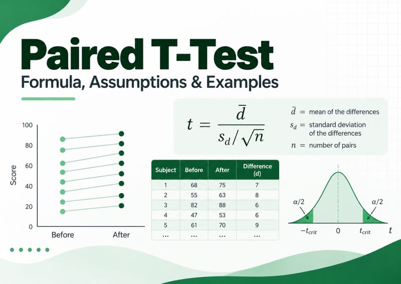
A paired t-test is a statistical hypothesis test used to determine whether the population mean difference between two related measurements is significantly different from zero.
For example, suppose a researcher measures the reaction time of the same participants before and after a training program. Since each participant provides two related measurements, the researcher can use a paired t-test to determine whether reaction time changed after the training.
The paired t-test does not treat the two sets of measurements as independent samples. Instead, it calculates a difference for every pair and tests whether the population mean of these differences is equal to zero.
In this guide, we explain when to use a paired t-test, its hypotheses and assumptions, the paired t-test formula, and how to calculate the test by hand using raw and summary data.
Already know how the test works and want to perform the calculation using your own data? Use our Paired T-Test Calculator.
What Is a Paired T-Test?
A paired t-test is a statistical test that compares two related measurements by analyzing the difference between each pair of observations.
Suppose the same 10 students take an examination before and after completing a training program. Each student’s before score is naturally paired with that student’s after score.
If we define the difference as d = Before − After, we obtain one difference score for every student. The paired t-test then asks whether the population mean of these differences, μd, is significantly different from zero.
Therefore, although two sets of measurements are collected, the statistical test is performed on a single sample of difference scores.
This is why a paired t-test is mathematically similar to performing a one-sample t-test on the paired differences, with the hypothesized population mean difference usually set to zero.
You may also see the paired t-test referred to as a dependent-samples t-test, dependent t-test, matched-pairs t-test, paired-samples t-test, or repeated-measures t-test.
When to Use a Paired T-Test
Use a paired t-test when you want to compare two related measurements of a quantitative variable. The observations must have a meaningful one-to-one relationship.
The table below shows some common situations where pairing occurs.
| Situation | Example |
|---|---|
| Before-and-after measurements | Blood pressure before and after treatment |
| Repeated measurements | Examination scores before and after a workshop |
| Two conditions applied to the same subjects | Reaction time under Condition A and Condition B |
| Matched individuals | Matching patients by age and comparing two treatments |
| Two methods applied to the same item | Measuring the same product using two instruments |
In each case, one observation in the first set corresponds directly to one observation in the second set.
Therefore, the key question is not simply whether you have two sets of data. You need to determine whether the observations are related.
For example, if 20 students take a test before and after training, use a paired t-test. However, if one group of 20 students receives Method A and a different group receives Method B, the observations are independent. In that case, you should use an Independent Samples T-Test instead.
Hypotheses
The paired t-test evaluates the population mean difference, denoted by μd. In the usual test, the null hypothesis assumes that the population mean difference is zero: H₀: μd = 0
However, the alternative hypothesis depends on the research question and whether the test is two-tailed, right-tailed, or left-tailed. The table below shows the research question and corresponding hypotheses for each type of paired t-test.
| Type of Test | Research Question | Null Hypothesis | Alternative Hypothesis |
|---|---|---|---|
| Two-tailed | Are the paired measurements different? | H₀: μd = 0 | H₁: μd ≠ 0 |
| Right-tailed | Is the mean difference greater than zero? | H₀: μd = 0 | H₁: μd > 0 |
| Left-tailed | Is the mean difference less than zero? | H₀: μd = 0 | H₁: μd < 0 |
As shown in the table, the null hypothesis remains the same in all three cases. What changes is the alternative hypothesis.
Before stating a directional hypothesis, you should also define how the paired difference is calculated. For example, d = Before − After and d = After − Before produce differences with opposite signs. As a result, the mean difference and t statistic will also have opposite signs. For a two-tailed test, however, the p-value will remain the same.
Therefore, you should use a two-tailed test when you want to determine whether a difference exists in either direction. However, if the research question specifies the expected direction of the difference before the data are examined, use a one-tailed test (left or right-tailed) instead.
Assumptions
Before performing a paired t-test, make sure the study design and data satisfy the assumptions of the test. Some of these assumptions are determined from how the data were collected, while others should be checked using the paired differences.
1. The Dependent Variable Should Be Quantitative
The variable being compared should be numerical and measured on a scale where calculating a mean is meaningful. Examples of quantitative variables include examination scores, blood pressure, weight, reaction time, temperature, and income.
For example, if you want to compare students’ examination scores before and after a training program, a paired t-test may be appropriate because the outcome is numerical.
However, a paired t-test is generally not appropriate for categorical outcomes such as pass/fail, yes/no, or treatment group. This assumption does not require a statistical test. You can determine whether it is satisfied by checking how the dependent variable was measured.
2. The Observations Must Be Paired
Each observation in the first set of measurements must have a meaningful match in the second set. This commonly occurs when the same individuals are measured twice. For example, a participant’s blood pressure before treatment should be paired with that same participant’s blood pressure after treatment.
Pairing can also occur when different individuals are deliberately matched on important characteristics, such as age or another relevant factor.
You should not create pairs simply because two groups contain the same number of observations. If one group of students uses Method A and a different group uses Method B, the observations are independent rather than paired. In that case, an Independent Samples T-Test would normally be more appropriate.
This assumption is checked from the study design rather than through a statistical test.
3. The Pairs Should Be Independent of One Another
The two measurements within each pair are expected to be related. However, each pair should be independent of the other pairs. For example, Participant 1’s before and after measurements form one pair. Those measurements should not determine or directly influence the measurements obtained from Participant 2.
Problems can arise when the same person appears in several supposedly separate pairs or when observations are clustered in a way that creates additional dependence between pairs.
There is usually no simple statistical test for this assumption. Instead, you assess it by considering how the sample was selected and how the measurements were collected.
If the data contain a more complicated dependence structure, such as several measurements from the same participants over time, another method such as a Repeated-Measures ANOVA may be more appropriate.
4. The Paired Differences Should Be Approximately Normally Distributed
The normality assumption applies to the difference scores, not necessarily to the two original variables separately.
Suppose we define the difference as: d = Before − After. You should first calculate a difference for every pair and then examine the distribution of those differences.
For example, if you have 20 before-and-after measurements, you will obtain 20 difference scores. It is these 20 values that should be approximately normally distributed.
You can check this assumption using a histogram, Q-Q plot, or Shapiro-Wilk test.
A histogram should show a reasonably symmetric distribution without severe skewness. In a Q-Q plot, the points should fall reasonably close to the diagonal reference line.
For the Shapiro-Wilk test, the hypotheses are:
- H₀: The difference scores are normally distributed.
- H₁: The difference scores are not normally distributed.
If the p-value is greater than the chosen significance level, such as 0.05, there is not enough evidence to reject the assumption of normality. A small p-value suggests that the difference scores depart from a normal distribution.
However, you should not rely on the Shapiro-Wilk test alone. With large samples, even small departures from normality may produce a significant result. It is better to consider the test together with a histogram or Q-Q plot.
Normality is generally more important when the number of pairs is small. With larger samples, the paired t-test is usually less sensitive to moderate departures from normality.
5. The Difference Scores Should Not Contain Extreme Outliers
Extreme outliers in the paired differences can have a strong effect on the mean difference, standard deviation, and t statistic. For this reason, you should examine the difference scores before performing the test.
A boxplot is one of the simplest ways to identify potential outliers. Values that appear far away from the rest of the observations should be investigated before continuing with the analysis.
However, you should not automatically remove a value simply because it appears as an outlier. First check whether it resulted from a data-entry or measurement error. If the value is genuine, consider whether it is reasonable to retain it and whether it has a substantial effect on the results.
If the difference scores contain severe outliers or are strongly non-normal, particularly with a small sample, the Wilcoxon Signed-Rank Test may be considered as a nonparametric alternative to the paired t-test.
Paired T Test Formula
The test statistic formula for a paired t-test is:
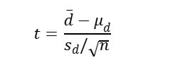
Where:
- t is the paired t-test statistic
- d̄ is the sample mean difference
- μd is the hypothesized population mean difference (usually 0)
- sd is the sample standard deviation of the differences
- n is the number of matched pairs
How to Perform a Paired T Test by Hand
A paired t test can be completed using the following six steps:
- State the null and alternative hypotheses.
- State the significance level.
- Calculate the test statistic.
- Find the p-value and critical value.
- Make the statistical decision.
- Write the conclusion in the context of the question.
In the next section, we demonstrate how to perform a paired t-test using the above steps using raw data and summary data examples.
Example 1: Raw Data
A researcher wants to determine whether a short training program changes reaction time. The same 10 participants complete a reaction-time task before and after training. Reaction time is measured in milliseconds.
| Participant | Before | After |
|---|---|---|
| 1 | 310 | 298 |
| 2 | 295 | 289 |
| 3 | 322 | 310 |
| 4 | 305 | 300 |
| 5 | 288 | 281 |
| 6 | 315 | 307 |
| 7 | 299 | 295 |
| 8 | 330 | 317 |
| 9 | 301 | 296 |
| 10 | 318 | 309 |
At the 0.05 significance level, is there evidence that the population mean reaction time changed after training?
Solution
Because the same participants were measured before and after training, the observations are related. Therefore, a paired t test is appropriate.
To perform the test manually, follow these steps:
Step 1: State the Hypotheses
The researcher wants to determine whether reaction time changed in either direction. Therefore, this is a two-tailed test.
The hypotheses are:
- H0: μd = 0
- H1 μd ≠ 0
Step 2: State the Significance Level
From the question, the significance level, α = 0.05
Step 3: Calculate the Test Statistic
By definition, the paired t test formula is: t = (d̄ -μd)/(sd/√n)
From the formula, we need to find the mean and standard deviation of the differences. To do that, follow these sub-steps:
i) Find the differences
Here, find the differences by subtracting the after scores from the before scores. The results are shown in the table below.
| Participant | Before | After | d = Before − After |
|---|---|---|---|
| 1 | 310 | 298 | 12 |
| 2 | 295 | 289 | 6 |
| 3 | 322 | 310 | 12 |
| 4 | 305 | 300 | 5 |
| 5 | 288 | 281 | 7 |
| 6 | 315 | 307 | 8 |
| 7 | 299 | 295 | 4 |
| 8 | 330 | 317 | 13 |
| 9 | 301 | 296 | 5 |
| 10 | 318 | 309 | 9 |
ii) Find the mean of the difference
The mean of the difference will give us d̄
Therefore, d̄ = (12+6+12+5+7+8+4+13+5+9)/10
=81/10
= 8.1
Alternatively, you can easily find the average of the differences using the average calculator.
iii) Find the sample standard deviation of the differences
By definition, the sample standard deviation formula is: s = √(Σx2 – nx̄2)/(n-1)
Σx2 is equivalent to finding the sum of all squared differences. Thus, Σx2 = 122+62+122+52+72+82+42+132+52+92
=753
You can also confirm the value using the sum of squares calculator.
Now, we can compute the sample standard deviation of the differences as follows: sd =√(753-10(8.1)2/(10-1)
=√10.76667
=3.28126
Want to instantly get the sample standard deviation without a manual process? Use the sample standard deviation calculator for an instant answer and step-by-step explanation.
iv) Find the test statistic
Recall, the paired t statistic formula is t = (d̄ -μd)/(sd/√n)
Substituting the values into the formula and solving, we get:
t = (8.1-0)/(3.28126/√10)
=8.1/1.0376
=7.8063
Recall. sd/√n can also be referred to as the standard error of the mean difference. You can actually compute this part by pasting the differences in the standard error calculator and clicking the calculate button.
Step 4: Find the P-Value and Critical Value
To find the p-value, you need the test statistic and degrees of freedom. For a paired t-test, the degrees of freedom formula is: df=n-1, where n is the number of matched pairs.
Since there are 10 matched pairs, then n = 10. Therefore, df = 10-1
= 9.
You can also verify this using the degrees of freedom calculator. Since this is a two-tailed test, you can use the following Excel formula to get the p-value =T.DIST.2T(ABS(7.8063), 9). Alternatively, using the p-value calculator from t, the two-tailed p-value for the test is: 0.000027
For the critical value, you need to use a t table and look up the value at: t0.05/2, 9 = ±2.2622. Alternatively, you can instantly get the same critical value using the critical t value calculator.
Step 5: Make the Decision
Since the p-value (0.000027) is less than the 0.05 significance level, we reject the null hypothesis. Also, the test statistic (7.8063) is greater than the absolute critical value (2.2622), we reject the null hypothesis.
Step 6: Write the Conclusion
At the 0.05 significance level, there is sufficient evidence to conclude that the population mean reaction time changed after training.
How to Calculate a Paired T-Test by Hand from Summary Data
Sometimes a question does not provide every original observation. Instead, you may already know the mean difference, standard deviation of the differences, and number of matched pairs.
In this situation, you can calculate the paired t-test directly without reconstructing the original measurements.
Example 2: Summary Data
A school recently introduced a test-preparation workshop and wants to know if it actually helps improve student performance. To find out, the exact same group of 16 students took an examination both before and after completing the workshop. When tracking individual progress (d = After score – Before score), researchers found that the average improvement was 3.6 points, with a sample standard deviation of 4.8 points. At a 0.05 significance level, is there enough evidence to prove that the workshop significantly changes overall examination scores?
Solution
From the question, we have summary data for the paired differences. In particular, we know that:
- Mean of the paired differences, d̄ = 3.6
- Sample standard deviation of the paired differences, sd = 4.8
- Number of matched pairs, n = 16
To conduct the paired t test manually using the summary data, follow these steps.
Step 1: Hypotheses
The researcher wants to determine whether examination scores changed in either direction. Therefore, this is a two-tailed paired t test.
The hypotheses are:
- H₀: μd = 0
- H₁: μd ≠ 0
Here, μd is the population mean of the differences between the after-workshop and before-workshop scores.
Step 2: Significance Level
From the question, we need to test the hypothesis at the 0.05 significance level. Thus, α = 0.05
Step 3: Test Statistic
By definition, the test statistic formula for a paired t test is:
t = (d̄ − μd)/(sd/√n)
Under the null hypothesis: μd = 0
Therefore, the formula becomes: t = d̄/(sd/√n)
Substituting the values into the formula, we get: t = 3.6/(4.8/√16)
= 3.6/1.2
= 3.00
Step 4: P-Value and Critical Value
Using the p-value from the t calculator or the p-value calculator, the two-tailed p-value for the test is 0.008973. Alternatively, you can find the p-value using the Excel formula: =T.DIST.2T(ABS(3.00), 15), where 15 is the degrees of freedom for the test, and 3.00 is the test statistic.
For the critical value, we need to find t0.05/2, 15 using the t-distribution table. This gives ±2.1314. However, if you prefer quick results, our t critical value calculator will yield a similar result.
Recall that 15 is the number of degrees of freedom for the paired t test. It is calculated using the formula: df = n − 1, where is the number of matched pairs. Thus, df = 16-1 = 15
Step 5: Decision
Since the p-value (0.008973) is less than the significance level (0.05), we reject the null hypothesis.
Alternatively, since the absolute test statistic (3.0000) is greater than the absolute critical value (2.1314), we reject the null hypothesis.
Step 6: Conclusion
At the 0.05 significance level, there is sufficient evidence to conclude that the workshop changes the population mean examination score.
Confidence Interval
In addition to testing whether the population mean difference is significantly different from zero, you can calculate a confidence interval for the population mean difference. The interval shows a range of plausible values for the true mean difference between the paired measurements.
The confidence interval formula for a paired t-test is:
CI = d̄ ± tcritical × (sd / √n)
where:
- d̄ is the sample mean difference.
- tcritical is the critical t value for the selected confidence level and degrees of freedom.
- sd is the standard deviation of the paired differences.
- n is the number of matched pairs.
Example.
From Example 1, we know that
- Mean difference, d̄ = 8.1
- Standard deviation of the differences, sd = 3.2813
- Number of pairs, n = 10
- Degrees of freedom, df = 9
From the above data, we can construct a 95% confidence interval as follows:
- Find the t-critical value. Using the t-table, the t-critical value, t.05/2, 9 = 2.2622.
- Substitute the values into the confidence interval formula and solve
Substituting these values into the confidence interval formula, we get:
CI = 8.1 ± 2.2622 × (3.2813 / √10)
= 8.1 ± 2.3473
Therefore, 95% CI = [5.7527, 10.4473]. You can verify this result or calculate the interval directly from your own raw or summary data using our Paired T-Test Confidence Interval Calculator.
We can interpret this interval to mean that the population mean difference is estimated to lie between approximately 5.75 and 10.45 milliseconds.
We can also use the confidence interval to make a decision about the hypothesis. In this case, since the 95% confidence interval does not contain zero, we reject the null hypothesis. This is consistent with the decision we made in Example 1.
Effect Size
A statistically significant paired t-test tells you that there is sufficient evidence of a population mean difference. However, statistical significance alone does not tell you whether that difference is small or large.
For this reason, it is useful to report an effect size alongside the p-value. A common effect size for a paired t-test is Cohen’s dz, which expresses the mean paired difference in standard deviation units.
The effect size formula is:
Cohen’s dz = d̄ / sd
where:
- d̄ is the sample mean of the paired differences.
- sd is the standard deviation of the paired differences.
Using Example 1, the mean difference was 8.1 and the standard deviation of the differences was 3.2813.
Therefore, Cohen’s dz = 8.1 / 3.2813
= 2.4686
The absolute value of Cohen’s dz can be interpreted using the following general guidelines:
- 0.2 indicates a small effect.
- 0.5 indicates a medium effect.
- 0.8 or greater indicates a large effect.
Since |2.4686| is greater than 0.8, the result in Example 1 represents a large effect.
The sign of Cohen’s dz indicates the direction of the mean difference. In this example, the differences were calculated as Before − After. As such, the positive effect size indicates that the before-training reaction times were higher than the after-training reaction times on average. If the subtraction order were reversed, the effect size would have the same magnitude but a negative sign.
These benchmarks should be treated as general guidelines rather than strict rules. The practical importance of an effect depends on the subject area and the context of the study.
How to Interpret a Paired T-Test
When interpreting a paired t-test, start with the mean difference rather than jumping straight to the p-value.
In Example 1, the mean difference was 8.1 milliseconds, where the differences were calculated as Before − After. This tells us that reaction times were, on average, 8.1 milliseconds higher before training than after training. The standard deviation of the differences was 3.2813, which shows how much the individual changes varied around this average difference.
We then look at the t statistic and p-value to determine whether the observed mean difference is statistically significant. In this example, t(9) = 7.81, p < .001. Since the p-value is less than the 0.05 significance level, we reject the null hypothesis and conclude that there is sufficient evidence that the population mean reaction time changed after training.
The 95% confidence interval for the mean difference was [5.75, 10.45]. Since zero is not included in this interval, it supports the same conclusion as the hypothesis test. It also suggests that the true mean reduction in reaction time is likely to fall within this range.
Finally, Cohen’s dz was 2.47, which indicates a large effect based on the commonly used guidelines. Therefore, the result is not only statistically significant but also represents a large difference relative to the variability in the paired differences.
How to Report a Paired T-Test in APA Style
When reporting a paired t-test, include the descriptive statistics for the two measurements when available, followed by the t statistic, degrees of freedom, p-value, confidence interval, and an effect size where appropriate.
Using Example 1, the before-training scores had: M = 308.30, SD = 13.08 while the after-training scores had: M = 300.20, SD = 10.78
Therefore, an APA-style report for this example could be written as:
A paired-samples t-test showed that reaction time was significantly higher before training (M = 308.30, SD = 13.08) than after training (M = 300.20, SD = 10.78), t(9) = 7.81, p < .001, 95% CI [5.75, 10.45], Cohen’s d = 2.47.
You should also explain the finding in the context of the research question. For this example, the result provides evidence that the training program was associated with a change in reaction time.
Struggling to report the paired t-test results in APA? Our Paired T-Test Calculator automatically generates an APA-formatted result, which you can copy and paste in your work.
Paired T-Test vs Independent T-Test
The paired and independent t-tests both compare means, but they are used for different types of data. A paired t-test is used when the observations are related, while an independent t-test is used when the observations come from separate, unrelated groups.
The table below compares the two tests based on the relationship between observations, study design, quantity being tested, degrees of freedom, and variance assumptions.
| Feature | Paired T-Test | Independent T-Test |
|---|---|---|
| Observations | Related | Unrelated |
| Typical design | Within-subjects | Between-subjects |
| Example | Same students before and after training | Different students taught using two methods |
| Main quantity tested | Mean of paired differences | Difference between two independent population means |
| Degrees of freedom | n − 1 | Depends on the independent t-test version |
| Equal variance assumption | Not required | Required for the pooled independent t-test |
As you can see from the above table, the main difference is whether the observations are related or independent. Therefore, you should use a paired t-test when each observation in one set has a meaningful match in the other set. However, if the two groups contain different, unrelated observations, use an Independent Samples T-Test instead.
Frequently Asked Questions
A paired t-test is a statistical test that determines whether the population mean difference between two related measurements is significantly different from zero.
Use a paired t-test when you have two related measurements, such as before-and-after observations from the same participants or matched pairs.
The degrees of freedom are calculated as df = n − 1, where n is the number of matched pairs.
Not necessarily. The main normality assumption applies to the paired differences rather than to each original measurement separately.
A paired t-test analyzes related observations, while an independent t-test compares two separate and unrelated groups.
Yes. If you have the individual difference scores, you can test whether their population mean is equal to zero. This is mathematically equivalent to a one-sample t-test on the paired differences.
